Att-GCN+MCTS [2021] Generalize a Small Pre-trained Model to Arbitrarily Large TSP Instances

Author: Zhen, TONG 2023-12-21

https://arxiv.org/pdf/2012.10658.pdf

Acknowledgments go to Prof. Zha and his dedicated students. This paper, a product of research conducted at my alma mater, The Chinese University of Hong Kong, Shenzhen, found its place in the prestigious 2021 AAAI publication.

Within these pages, the authors introduce an innovative concept—the fusion of Supervised Learning (SL) and Reinforcement Learning (RL).

Method

This research is specifically tailored for the Euclidean space Traveling Salesman Problem (TSP). Initially, the Supervised Learning (SL) component takes charge, producing a graph's heatmap. This heatmap represents a probability output assigned to each edge, as formally described below:

P_{ij}\in[0, 1]

The probability ($P_{ij}$) signifies the likelihood of an edge existing between nodes $i$ and $j$. The researchers adopted an off-line learning approach, training a graph convolutional residual neural network with attention mechanisms—abbreviated as Att-GCRN. This model was trained on 990,000 instances of the Traveling Salesman Problem (TSP), leveraging Concorde as a solver for labels.

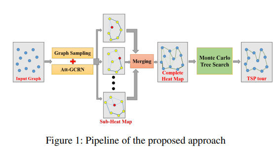
Upon completing the training of the Graph Convolutional Network (GCN) or Graph Neural Network (GNN) for smaller graphs, the team proceeded to sample sub-graphs from larger graphs. For these smaller graphs, they generated individual heatmaps, merging them subsequently into a comprehensive heatmap. Finally, to search for high-quality TSP solutions, guided by the information encoded in the consolidated heatmap, they employed Monte Carlo tree search (MCTS).

Sub-Graph Sampling

The sampling process is intuitively straightforward. When dealing with a graph, one can simply randomly select the least visited nodes, edges, and their k-nearest neighbor nodes. This involves utilizing a visitation variable, denoted as $O_i$ or $O_{ij},$ to keep track of the frequency of visits to each node or edge. The heat map is then calculated based on these visitation records. This iterative process continues until a predetermined threshold is reached. Additionally, the graph conversion step, which essentially entails a scale transformation for the sub-graph, is a straightforward operation.

Merging

The story sounds good so far, except for the emerging step. Actually, it is also very easy:

P_{ij} = \frac{1}{O_{ij}}\sum_{l = 1}^I P''_{ij}(l)

Reinforcement learning for solutions optimization

They use the action of k-opt, which is to delete k edges in the solution state and add k edges to the new solution state. Afraid of making an infeasible solution, they take a way called the compact method.

They first search the action in a small neighborhood i.e. k = 2. then enlarge the neighborhood with RL, because the searching space can be too big.

The motivation for the MCTS is for the big search space (state space), the main idea of MCTS is first to take a limited depth of searching tree, then simulate the whole trajectory by a few samples, and estimate the whole space with the Monte-Carlo Method. To balance the exploration and exploitation, it uses the UCB method, which counts the state visit times, and the estimated value. This paper is just doing the same thing using matrix $W, Q$ , corresponding to the estimated value, and visit times, but especially in graph problems, therefore their dimension is nxn. They are called the weight matrix and access matrix,(initialized to 0) and record the times that edge (i, j) is chosen during simulations. Additionally, a variable M (initialized to 0) is used to record the total number of actions already simulated.

As explained before, each action is represented as $a = (a_1, b1, a_2, b_2, . . . , a_k, b_k, a_{k+1})$ , vontaining a series of sub-dicisions $a_i$ , $1 ≤ i ≤ k$ ( $k$ is also a variable, and $a_{k+1} = a_1$ ), while $b_i$ could be determined uniquely once $a_i$ is known.

In the simulation step, they use a variable called potential $Z_{b_{i,j}}$ , basically the UCB form in the graph for doing MCTS. The higher the value of $Z_{b_{i}, j}$ , the larger the opportunity of edge $(b_i, j)$ to be chosen:

Z_{b_i, j} = \frac{W_{b_i, j }}{\Omega_{b_i}}+\alpha\sqrt{\frac{\ln(M+1)}{Q_{b_i, j}+1}}

\Omega_{b_i} = \frac{\sum_{j\neq b_i}W_{b_i, j}}{\sum_{j\neq b_i}1}

$\Omega_{b_i}$ is an averaged $W_{b_i, j}$ of all the edges relative to vertex $b_i$ . After the leaf node in the MCTS is selected, then rollout, which is called the sub-decisions in the paper. Randomly choosing action $a_i$ , and action the determined $b_i$ . Finally, backpropagate the rollout, and update the probability of choosing the vertices as:

P_j = \frac{Z_{b_i, j}}{\sum_{l\in\mathbb{X}}Z_{b_i, l}}

$\mathbb{X}$ is all the leaf candidate nodes for the next edge to connect. If any vertices of $b_i$ are in an improving state, keep it; otherwise, randomly choose one $(b_i, j)$ . Whenever a state action pair is examined, backpropagate the $W_{i, j}$ weight matrix

W_{b_i, a_{i+1}}\leftarrow W_{b_i, a_{i+1}}+\beta[\exp{(\frac{L(s)-L(s_{new})}{L(s)})-1}]\\Q_{b_i, a_{i+1}}\leftarrow Q_{b_i, a_{i+1}}+1

Experiment

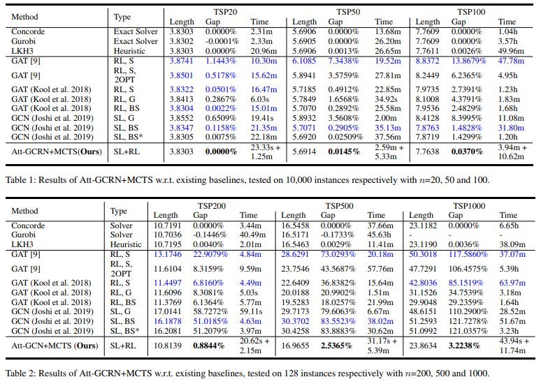
According to the experiment of the paper, they are very close to Concord with way faster speed.